Aligning Planning Models with Real-World Observations

Motivation

As humans, we reason about our surrounding environments with prior common-sense knowledge that influences our understanding. For example, the expectation that an object will fall when dropped due to gravity, or the understanding that objects cannot teleport or instantly vanish. Ideally, artificial intelligence systems should have this understanding as well. Consider a sequence of images showing a robot moving between rooms: in this work, we want to predict the state of the environment in each frame, and we also have an understanding of what transitions are feasible in this environment. We assume that in between frames the robot can move to an adjacent room, but cannot suddenly teleport to an unconnected room. The problem is then to predict the states of these images in a manner that adheres to our expectations for how the environment behaves.

Problem setting

In this work, we aim to improve the predictions of a computer vision model through aligning a sequence of images and their predictions with a graph representing how the system can transition between states. This problem is highlighted below.

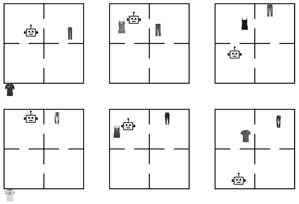
On the left is an example of the kind of data we’re looking at: sequences of images showing actions taking place in an environment. These are examples of the images the computer vision model is predicting the underlying state of. In this environment, the actions are the agent picking up objects (represented by the number 0 for this example) and moving between rooms. The robot can pick up the object (represented by the object moving to the bottom left corner outside the rooms) and place it in the robots current room. The idea is that the state should be recognized as being the same no matter where in the room the robot or the object is located - all that matters is the room they are in. Furthermore, the appearance of the object changes between states - we sample this from the MNIST dataset of handwritten numbers to obtain variation.

The graph on the right shows the state space - this is essentially a model of how we know the environment to behave. The state of the image on the left is highlighted in grey. In this graph, there is an edge from one state to another if there is a valid transition between those states, in this case if there is an action in the corresponding planning domain of the problem that transitions from one state to the other. Given the sequence of images such as those shown on the left in the gif, we expect that the corresponding states form a path in the graph. That is, there is a valid transition occuring between each sequential pair of states in the sequence.

Goal

Given a sequence of images representing states in a given state-space, we want to train a model to predict the underlying state for each image. Futhermore, we want the sequence of predictions to align with a given state-space graph that dictates which transitions are valid in the environment.

The data

First, we generate some data using planning domains as a testbed.

Here, both rows show a sequence of the same 3 states. In these examples the objects are sampled from the Fashion MNIST dataset, each object represented as a different item of clothing. Each image on the top is the same state as the one below it, but visually they appear different due to sampling different items of clothing and the position of objects. The challenge here is for the model to learn concepts like “t-shirt” and “pants” to differentiate the objects, as well as understanding which room an object is in when the objects position in the room can change between states.

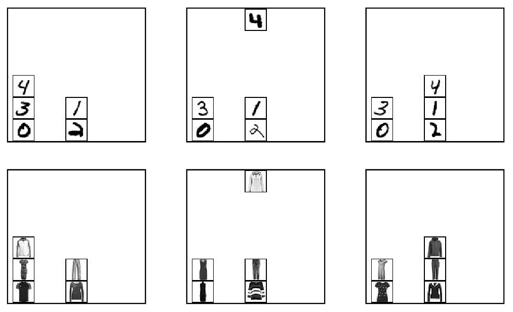
Here, labeled blocks are moved around on a table. The model needs to differentiate between the blocks, and understand what state the specific arrangement of blocks corresponds to. Above, the labels are numbers sampled from MNIST. Below, they are represented by different articles of clothing sampled from Fashion MNIST for increased difficulty.

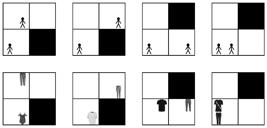
This domain models people taking an elevator, where they are shown waiting at different floors on the left half, and the elevator is shown on the right half. Above, we highlight the mechanics using stick figures, showing a person on the 2nd floor getting on the elevator and getting off at the first floor. Below shows what the equlivalent states look like in our training data: representing different people as different clothing items, and assigning them locations within the waiting area or elevator randomly to add difficulty disambiguating between states.

The model

To predict the state we use contrastive learning. This is a deep learning framework that aims to represent images belonging to the same class similarly, while distancing these representations from those of images belonging to a different class. In our case, examples of images representing the same underlying state should have representations that are similar, yet different and identifiable from representations of different classes. We experimented with several contrastive methods before deciding to use SupCon, of which the general architecture is depicted and described below.

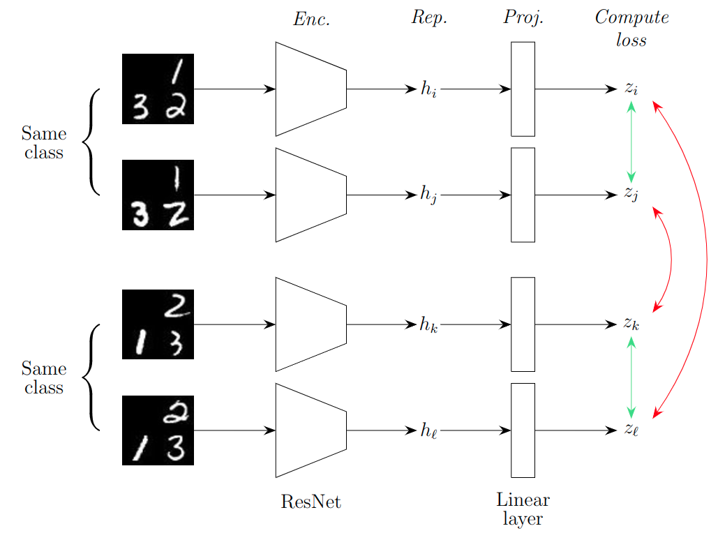
The first two images belong to the same class and hence should be represented similarly, as represented by the green arrow on the right which represents pulling the representations together. The bottom pair of states are also both the same, but different from the top two states. Hence, their representations should be different, as represented by the red arrows on the right side of the figure. The network has two parts, an encoder (‘Enc.’) and a projector (‘Proj.’). While the contrastive loss is applied on the output of the projector, the representation used for downstream tasks is the one after the encoder but before the projector, labelled as ‘Rep.’ in the figure.

Not shown in this figure is an additional linear layer after ‘Rep.’ (the $h$’s), this layer has an output neuron for every state in the state-space, acting as a classifier for the final state. We convert the output of this layer (without any activation functions applied) to a probability distribution to obtain the ‘probability’ of the input image representing each state.

Aligning algorithms

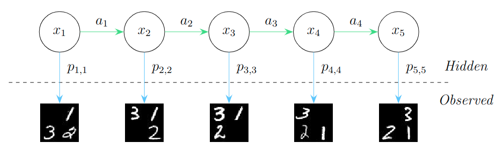
Below shows the general problem: the sequence of states $x_1, x_2, x_3, x_4, x_5$ is what we want to predict from the observations shown below. From the predictive model, we have for every state the probability that each prediction is that certain state, and we want to select the sequence of states that maximizes the probability of the observations being those states, while aligning the sequence of predictions with the underlying state space.

We test three alignment algorithms: a greedy approach, beam search, and Viterbi’s algorithm.

Greedy align

This method builds the solution in a greedy manner, starting from the beginning of the trace and aligning the predictions one edge at a time. The search is limited to the top-$n$ predictions for each observation, and if a connecting edge isn’t found at one step then the best edge between the next pair of observations is chosen. This allows the method to ‘come off track’ and select a sequence of predictions that may not fully align with the state space.

This can be seen in the gif above: first, the best edge between the first two observations is selected, then the method ‘continues the chain’ by selecting the next best connected edge. After this, there is no next connected edge in the top-$n$ predictions, so the algorithm skips over this edge and finds the best edge between the next two observations. This results in a sequence of states not fully aligned with the graph, but helps the algorithms ‘get back on track’. Restricting the search to the best top-$n$ helps prevent poor choices being made that encourage further errors.

Beam align

Beam search maintains $W$ solutions at each, where $W$ is the ‘beam width’. First, the top-$W$ predictions for the first observation are selected. Then, the corresponding nodes in the graph are expanded to obtain a set of all neighbouring nodes. These neighbouring nodes are all potential candidates for the prediction in the sequence. From this set, the top-$W$ are selected, extending whichever previous prediction they neighboured. If one node was the neighbour of more than one prediction for the previous observation, then the best previous prediction is the one continued on. After reaching the last observation, the path with the best joint probability over all observations is chosen.

This process is shown above. Note that for every observation, there are always $W$ nodes chosen to continue on from. In the paths maintained by the algorithm, each node only has one incoming edge, but may have multiple outgoing edges.

Viterbi align

Viterbi’s algorithm is an exhaustive approach that finds the optimal solution with respect to the probabilities given by the state prediction model, which itself may be flawed. It is essentially the same as the beam search algorithm shown, with the beam width parameter set to the number of states. For every state prediction for each observation, the algorithm maintains the best path up to that state for that observation. At the end the path with the highest joint probability is selected.

This process is shown above. At the end, the algorithm backtracks through the table to obtain the final sequence.

Results

Below we highlight the main results.

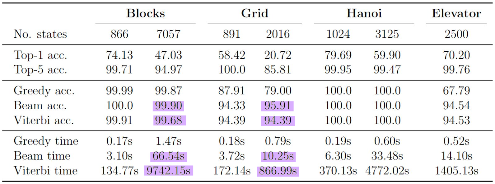
Here, top-1 accuracy represents the accuracy of the top prediction returned by the model, while top-5 accuracy represents how frequently the correct prediction was in the top-5 most likely predictions. Notably, top-5 accuracy is generally quite high, and generally significantly higher than the top-1 accuracy. This is the case even in domains with thousands of states. This result is interesting as it demonstrates that in many cases where the model does not predict the state correctly, the correct state is generally still ranked quite high by the model.

Next, in the Greedy accuracy, Beam accuracy, and Viterbi accuracy sections we report the accuracy after aligning the predictions with the state-space graph using the respective alignment algorithms. Generally, accuracy is significantly better than the original top-1 accuracy. The most surprising result is in all cases, Beam alignment outperforms Viterbi alignment, while taking only a small fraction of the time (shown highlighted in purple in the table). For the Blocks domain with 7057 states Beam align took ~1 minute and attained 99.9% accuracy, while Viterbi align took over 2.5 hours and only attained 99.68% accuracy.

While it’s not clear why Beam align outperforms Viterbi align, my hypothesis is that Beam align takes advantage of the phenomenon discussed previously - that the correct prediction is generally ranked quite high, with the majority generally being in the top-5 most likely predictions. Since Viterbi searches more exhaustively it could be prone to finding sequences that may appear more feasible, but the predictions are generally ranked lower. Since Beam searches more shallowly it restricts its search to more likely predictions, resulting in an ultimately more accurate trade-off between single prediction likelihood and alignment with the graph.

For more in-depth details and results, my thesis can be found here.