
Learning Graph Relationships in Spatiotemporal Data for Time Series Forecasting
My Role
My contributions to this project were in engineering, data processing and writing. Specifically, I collected and processed the synthetic, traffic, and bike sharing datasets (aside from Nice Ride Minnesota), refactored the code to make the full pipeline run smoothly, and set up experiments against other architectures (namely the ASTGCN network from [1]). I also assisted in the writing of the paper. The project was led by Ryan Zhou, first author on the paper.
Problem
Many real-world problems involve spatiotemporal data, which includes both spatial and time relationships. For instance, in applications such as traffic flow modeling, bike share network forecasting, disease modeling, and meteorology, activity at multiple spatial points must be considered. The applications we focus on are bike share networks and traffic flow modeling.
One of the biggest issues for a bike sharing system is distribution of bikes across stations, as stations can either run out of bikes or have more bikes than there are available docks. Spatiotemporal modeling is a vital tool to predict when and where redistribution is required in the bike network, something which is generally handled by system operators who must manually move bikes between stations. Thus, accurately predicting patterns can aid system management and improve the experience for end users. Predicting traffic flow is also of significant importance as understanding traffic flow is essential for urban planning and traffic management or control. Upstream roads will impact downstream roads due to the flow of traffic, and downstream roads impact upstream roads as drivers may try to avoid issues like traffic jams, construction, or accidents. This relationship is complex as an increased amount of activity at one location may impact activity in multiple locations in the future, creating a need for more advanced predictive systems.
Spatiotemporal forecasting requires a neural network to learn both time and space relationships. Many relationships are not purely spatial or purely temporal, but instead span both space and time. This type of diagonal relationship is common in sensor data; a physical event may be detected at one sensor, and later detected at another sensor, separated by a number of timesteps. In order to perform accurate forecasts, we would like the model to learn this time-delayed pattern which moves through space.
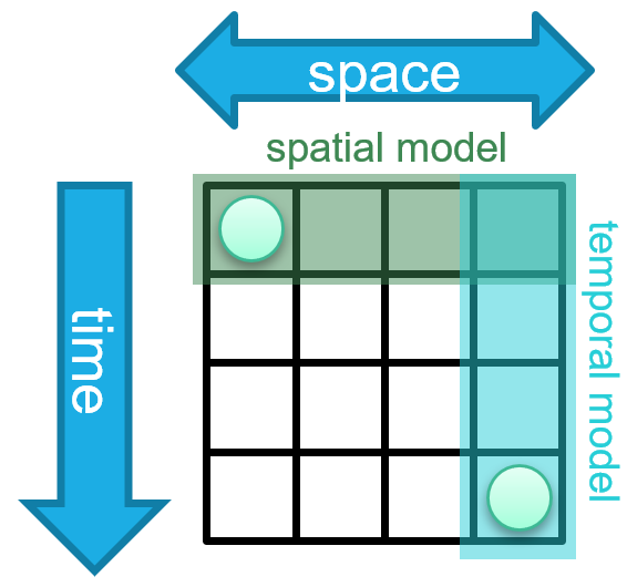
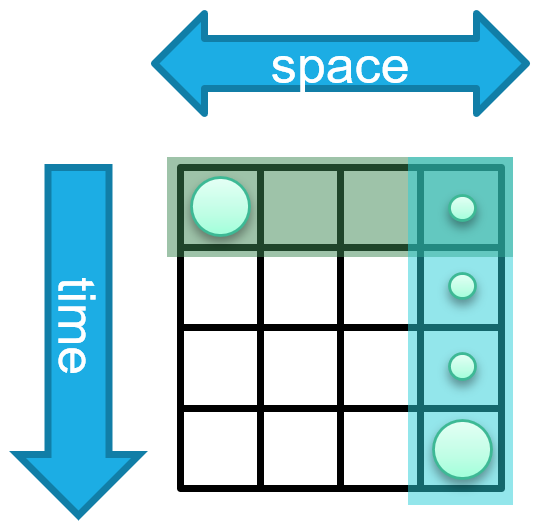
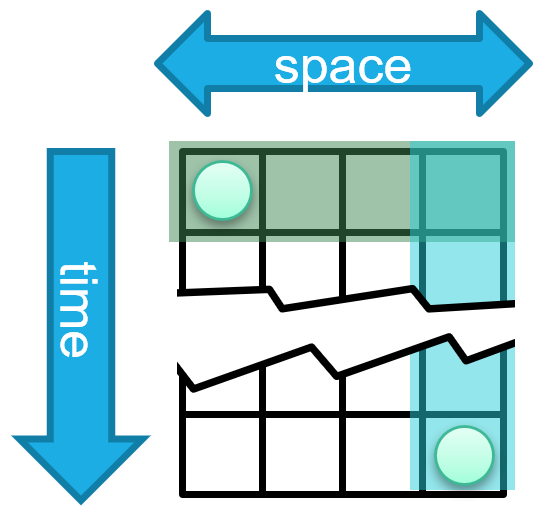
Figure 1: The spatiotemporal forecasting issue
A common approach is to use independent spatial and temporal layers which can capture each type of dependency and arrange the layers sequentially, allowing them to exchange information. Learning these diagonal dependencies requires the two models to coordinate with each other (Figure 1 left). However, because both models operate independently, it is necessary for the spatial model to diffuse information regarding the event before the temporal model can access it, or vice versa. This results in the temporal model being passed information regarding the event before it becomes relevant in the physical system, which may impact the predictions made by the temporal model or result in noise or leakage (Figure 1 middle). An intrinsically spatiotemporal layer avoids some of these problems; however, designing such a layer poses its own challenges. For high sampling rates, many timesteps may pass before the information is needed in comparison to the number of spatial hops (Figure 1 right). This requires the ability to handle long sequences without releasing information early.
Our Solution and Methodology
Our proposed solution is to add a separate graph memory state which deals solely with activity in other nodes, while leaving the original memory state (the primary memory) to model temporal dependencies in its own node. The output from the graph memory state is fed into the primary memory as determined by the graph memory’s output gate. This allows the temporal model to become “aware” of network events without directly impacting the output. In addition, feeding the graph memory into the main memory rather than the output ensures that events are directly incorporated into long-term memory, rather than needing to pass through the input gate at the next timestep.
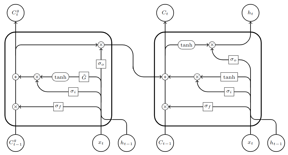
Figure 2: Our proposed model
The architecture of our proposed model is displayed in Figure 2. The block on the right contains a standard LSTM unit with no graph operations. The block on the left contains the added graph memory component which performs graph operations and stores results separately using its own set of gates. The output of the graph memory component feeds into the memory of the main (non-graph) LSTM unit, allowing spatial information to be introduced only when needed. The inputs $x_t$ and $h_{t-1}$ are the same for both units.
We test several different architectures for comparison. First, we include as baselines a purely temporal model (LSTM) with no spatial model, a purely spatial model (GCN) with no temporal model, and a combined model with alternating LSTM and GCN layers (GCN + LSTM). We next test a number of spatiotemporal models: two variants of graph LSTM (GLSTM) with different graph operations (GCN and GAT); ASTGCN, an attention-based spatiotemporal model [Guo et al., 2019]; and finally, two variants of our proposed graph memory LSTM (GM-LSTM) with different graph models (GCN and GAT). We use only the “recent” component of ASTGCN, denoted by ASTGCN$_r$, as only the most recent timesteps are available to all models.
Data
To explore the ability of models to learn spatiotemporal relationships over long timescales, we first evaluate our model on a synthetic dataset with variable difficulty. We then evaluate our model on 7 real-world datasets divided into two applications, bike sharing and traffic forecasting.
Synthetic
The synthetic path dataset is designed to test the ability of models to learn spatiotemporal dependencies over long time periods. This consists of a directed path graph, where each vertex in the graph has an edge pointing to the next vertex. Signals appear at random at the first node in the graph and propagate along the edges, with a variable delay for propagation. This is a common pattern in real-world sensor data, where events are first detected at one sensor before appearing at a second sensor. Depending on the sampling rate and the speed of propagation, there may be a delay of several timesteps before it is detected again. As the amount of delay increases, this pattern becomes increasingly difficult to predict; a neural network must be able to retain information of the previous signal without allowing it to affect outputs before the signal reappears.


Figure 3: Generated synthetic data with delays of 1, 3, and 8, respectively. The rows correspond to nodes in the network (where each square’s node is connected to the node to it’s right), the columns are the nodes over time, and their brightness corresponds to their magnitude. It can be best seen in the leftmost figure how the signals are propagating across the graph.
Bike Sharing
We use data from three different bike sharing systems: Nice Ride Minnesota, Citi Bike NYC, and Bluebikes Boston. This data consists of lists of trips, which we bin into hourly or daily activity counts and cast as time-dependent node features. We use these counts as the prediction targets. As additional features we include station capacity and timestamps, and weather information (Nice Ride) and geographic information (Bluebikes, Citi Bike) where available. To generate the graph, edges are placed between stations with a significant number of trips between them. Significance is determined by finding the mean number of incoming bikes from every other station, including itself. A directed edge is placed from the station to all stations which contribute an average or above number of incoming trips to the given station.
Traffic Forecasting
We use four traffic sensor datasets to evaluate models for this application. The Texas Traffic and Washington Traffic datasets consist of sensor data listing the number of vehicles that travelled past the sensor each hour (our prediction target), the direction of travel and coordinates of the sensor. Unlike bike data, individual trips are not logged; thus, we generate the graph for these two datasets by adding edges between sensors that are in close geographical proximity. The processed PeMSD4 and PeMSD8 datasets and graphs are provided by [Guo et al., 2019], and contain traffic data collected by Caltrans Performance Measure System (PeMS) in California, with the features ‘total flow’ (our prediction target), ‘average speed’, and ‘average occupancy’.
Results
Synthetic


Figure 4: From left to right, these are: target, LSTM, GCN, GLSTM, AST-GCN, GM-LSTM (ours). Each image should match the target image if predictions are 100% accurate.
Figure 4 shows sample predictions for various models on the path dataset with a delay of 20. As expected, the GCN alone lacks temporal information and produces poor predictions. The stacked GCN/LSTM model produces predictions noisier than those produced by the graph memory LSTM model. We attribute this to crosstalk between the spatial and temporal layers. In the graph memory model, the gating mechanism reduces this effect and predictions are qualitatively almost identical to the target.
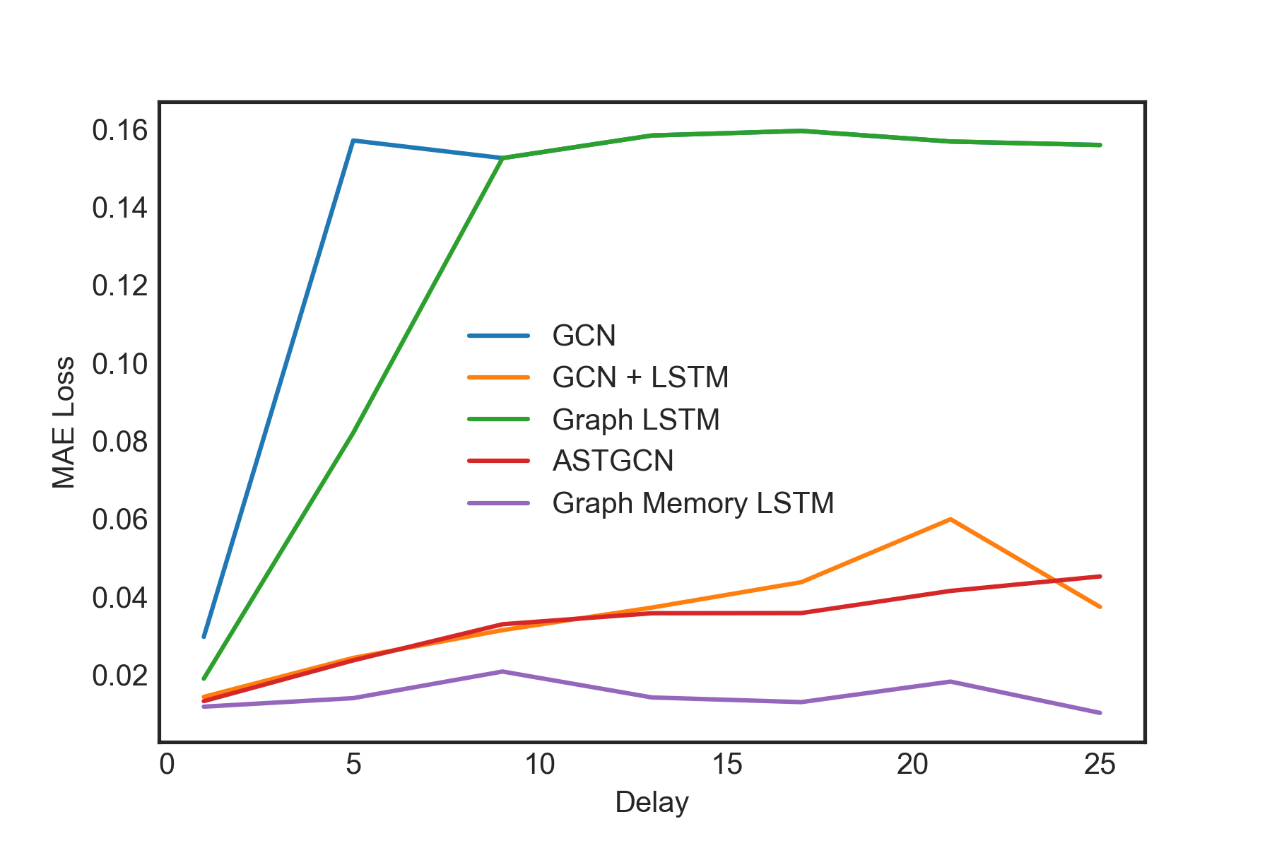
Figure 5: MAE of models on synthetic data as signal delay is varied. Error for most models increases as delay is increased; however, graph memory LSTM is able to learn these relationships without significant increase in error up to a delay of 25 timesteps
Results on the synthetic path dataset (Figure 5) show that as the delay time for signal propagation increases, this task becomes increasingly difficult for most architectures. After a sufficiently large delay, some models were altogether unable to learn the relationship. However, we see that the graph memory model has an increased ability to retain information about other nodes and performance is not appreciably degraded even up to a delay of 25 timesteps.
Traffic and Bike Sharing
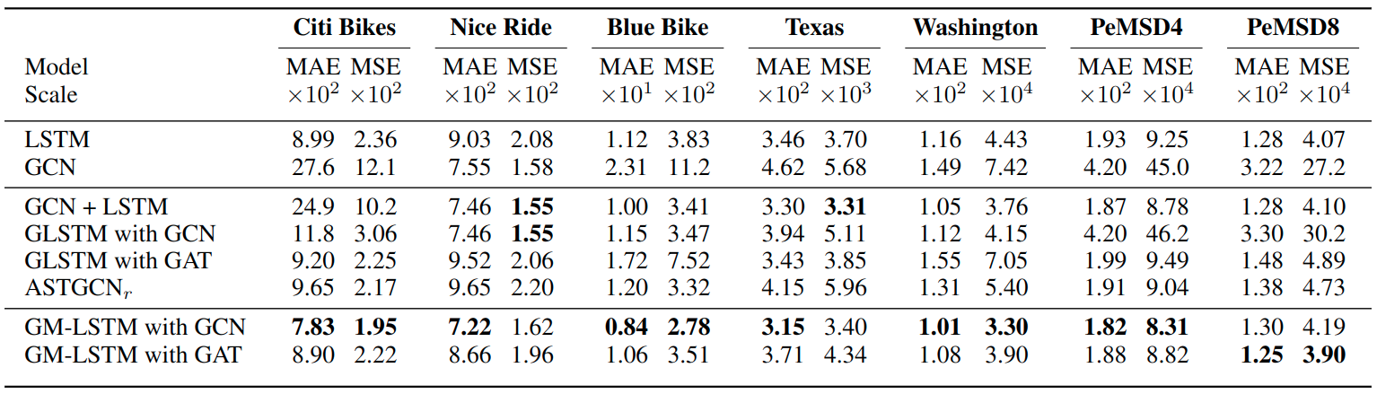
Table 1: Results for bike and traffic datasets multiplied by the scale column. Individual temporal and spatial models are listed first. GCN + LSTM denotes stacked GCN and LSTM layers. ASTGCN$_r$ denotes the “recent” component of the ASTGCN model as only the most recent timesteps are given as input to all models. GCN models use trainable edge weights.
We observe that in most cases the graph memory models outperform the other architectures tested, suggesting that the improved performance observed on the synthetic dataset also translates to benefits for real-world data. The difference was most pronounced on the traffic datasets due to the high degree of spatial and temporal correlation. On the Nice Ride bike dataset, when measured by mean squared error, other models achieve similar or better performance; we believe this is due to the binning by day reducing the effective time delay for the spatiotemporal dependencies. We also observe that for the spatiotemporal GLSTM and GM-LSTM models, the GCN variants with trainable weights generally outperform the GAT variants. We theorize this is due to the larger number of parameters in these models (corresponding to the size of the adjacency matrix) as well as the nature of the data, with relationships between stations remaining relatively constant across time due to their fixed physical positions. However, using fixed trainable weights may be impractical for large, dense graphs due to the number of parameters required.
References
[Guo et al., 2019] Shengnan Guo, Youfang Lin, Ning Feng, Chao Song, and Huaiyu Wan. Attention based spatial-temporal graph convolutional networks for traffic flow forecasting. In Proceedings of the AAAI Conference on Artificial Intelligence, volume 33, pages 922–929, 2019.